Propagation

Scripts to propagate the orbits

Propagation implemented by Walther Litteri

Tolerance Constants

Jacobi Constant

jacobi_constant

 jacobi_constant (X:numpy.ndarray, mu:float)

*State-dependent Jacobi constant for a given state vector X and gravitational parameter mu.

Parameters: X (np.ndarray): Cartesian state vector with 6 components (x, y, z, xp, yp, zp). mu (float): Gravitational parameter.

Returns: Tuple[float, float]: Jacobi constant (J) and total energy (E).*

	Type	Details
X	ndarray	Cartesian state vector with 6 components (x, y, z, xp, yp, zp)
mu	float	Gravitational parameter
Returns	Tuple

orbit_data = get_example_orbit_data()
orbit_data.shape

(400, 7, 100)

# Calculate Jacobi constants and energies for all orbits at all time points
jacobi_constants = np.zeros((400, 100))
total_energies = np.zeros((400, 100))

for orbit_index in range(400):
    for time_index in range(100):
        X = orbit_data[orbit_index, 1:, time_index]
        J, E = jacobi_constant(X, EM_MU)
        jacobi_constants[orbit_index, time_index] = J
        total_energies[orbit_index, time_index] = E

# Flatten the Jacobi constants array to plot the histogram of all values
jacobi_constants_all = jacobi_constants.flatten()

# Plot histogram of Jacobi constants for all orbits
plt.figure(figsize=(10, 5))
plt.hist(jacobi_constants_all, bins=50, color='blue', alpha=0.7)
plt.title('Histogram of Jacobi Constants for All Orbits')
plt.xlabel('Jacobi Constant')
plt.ylabel('Frequency')
plt.grid(True)
plt.show()

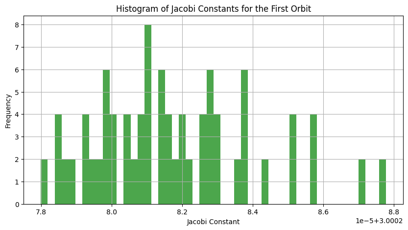
# Plot histogram of Jacobi constants for the first orbit
jacobi_constants_first_orbit = jacobi_constants[0, :]

plt.figure(figsize=(10, 5))
plt.hist(jacobi_constants_first_orbit, bins=50, color='green', alpha=0.7)
plt.title('Histogram of Jacobi Constants for the First Orbit')
plt.xlabel('Jacobi Constant')
plt.ylabel('Frequency')
plt.grid(True)
plt.show()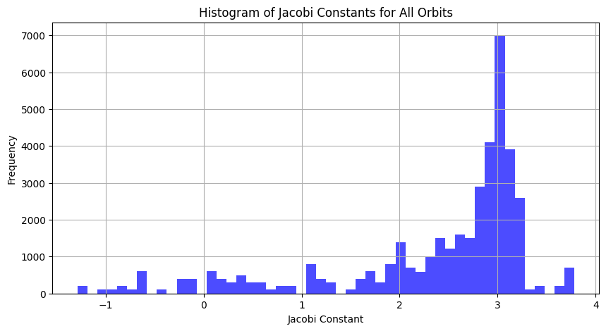

Equations of motion CR3BP

source

eom_cr3bp

 eom_cr3bp (t:float, X:numpy.ndarray, mu:float)

*Equations of motion for the Circular Restricted 3 Body Problem (CR3BP). The form is X_dot = f(t, X, (parameters,)). This formulation is time-independent as it does not depend explicitly on t.

Parameters: t (float): Time variable (not used in this formulation). X (np.ndarray): State vector with 6 components (x, y, z, v_x, v_y, v_z). mu (float): Gravitational parameter.

Returns: List[float]: Derivatives of the state vector.*

	Type	Details
t	float	Time variable (not used in this formulation)
X	ndarray	State vector with 6 components (x, y, z, v_x, v_y, v_z)
mu	float	Gravitational parameter
Returns	List

# Select a random orbit from the dataset
num_orbits, num_components, num_time_points = orbit_data.shape  # Now (400,7,100)
random_orbit_index = np.random.randint(0, num_orbits)
X0 = orbit_data[random_orbit_index, :6, 0]  # Take only first 6 components for state vector
mu = 0.01215058560962404
T0 = 2.7430007981241529E+0  # Total time for the propagation, can be adjusted as needed

# Propagate the orbit using solve_ivp
sol = solve_ivp(eom_cr3bp, [0, T0], X0, args=(mu,), dense_output=True, rtol=1e-9, atol=1e-9, method='Radau')
tvec = np.linspace(0, T0, num_time_points)
z = sol.sol(tvec)

# Compute derivatives using eom_cr3bp for a specific state in the propagated orbit
time_index = np.random.randint(0, num_time_points - 1)  # Choose a random time index
t = tvec[time_index]
X = z[:, time_index]
computed_derivatives = eom_cr3bp(t, X, mu)

# Compare with actual changes in state vector
delta_t = tvec[1] - tvec[0]
actual_derivatives = (z[:, time_index + 1] - z[:, time_index]) / delta_t

# Visualize the actual trajectory and computed derivatives
fig, axs = plt.subplots(2, 1, figsize=(10, 12))

# Plot the actual trajectory
axs[0].plot(z[0], z[1], label='Trajectory')
axs[0].scatter(z[0, time_index], z[1, time_index], color='red', label='Point of Interest')
axs[0].set_xlabel('x')
axs[0].set_ylabel('y')
axs[0].set_title('Trajectory in the XY plane')
axs[0].legend()
axs[0].grid(True)

# Plot computed vs. actual derivatives
labels = ['x_dot', 'y_dot', 'z_dot', 'x_ddot', 'y_ddot', 'z_ddot']
width = 0.3  # width of the bars
x = np.arange(len(labels))  # the label locations

axs[1].bar(x - width/2, computed_derivatives, width, label='Computed')
axs[1].bar(x + width/2, actual_derivatives, width, label='Actual')
axs[1].set_xticks(x)
axs[1].set_xticklabels(labels)
axs[1].set_xlabel('Derivative')
axs[1].set_ylabel('Value')
axs[1].set_title('Computed vs Actual Derivatives')
axs[1].legend()
axs[1].grid(True)

plt.tight_layout()
plt.show()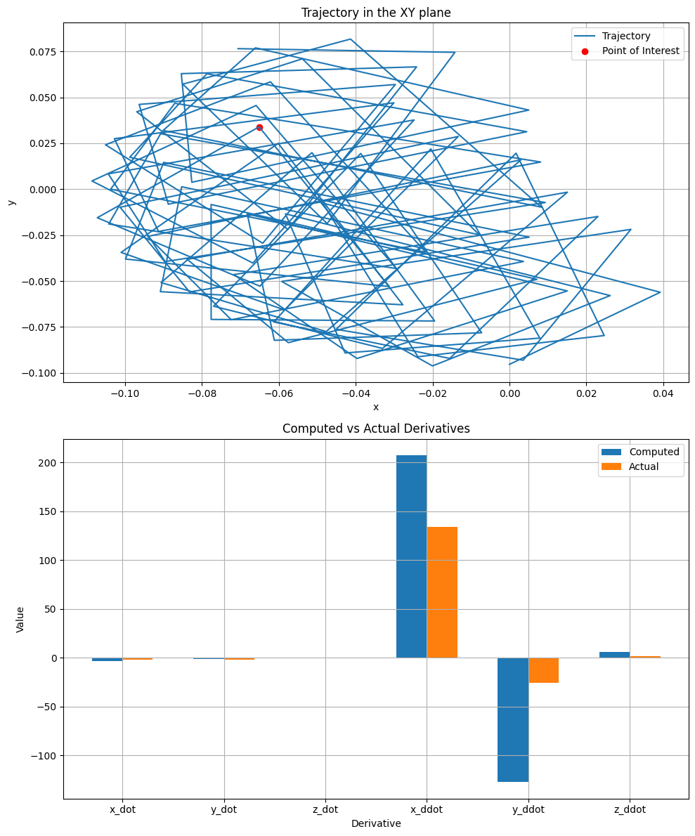

Propagation

source

prop_node

 prop_node (X:numpy.ndarray, dt:float, mu:float)

*Return the state X after a given time step dt = T_end - T_start.

Parameters: X (np.ndarray): Initial state vector with 6 components (x, y, z, v_x, v_y, v_z). dt (float): Time step for propagation. mu (float): Gravitational parameter.

Returns: np.ndarray: Final state vector after time step dt.*

	Type	Details
X	ndarray	Initial state vector with 6 components (x, y, z, v_x, v_y, v_z)
dt	float	Time step for propagation
mu	float	Gravitational parameter
Returns	ndarray

# Select a random orbit from the dataset
num_orbits, num_components, num_time_points = orbit_data.shape  # (400, 7, 100)
random_orbit_index = np.random.randint(0, num_orbits)
X0 = orbit_data[random_orbit_index, 1:, 0]  # Take components 1-6 (skip time)
mu = 0.01215058560962404
dt = 0.1  # Small time step for propagation

# Propagate the state vector using prop_node
X_final = prop_node(X0, dt, mu)

# Print the initial and final state vectors
print("Initial state vector:", X0)
print("Final state vector after time step dt:", X_final)

# To visualize the propagation, we can propagate over multiple time steps and plot the trajectory
T_total = 2.0  # Total time for propagation
time_steps = int(T_total / dt)
trajectory = np.zeros((time_steps + 1, 6))
trajectory[0] = X0

# Propagate step by step
X_current = X0
for i in range(1, time_steps + 1):
    X_current = prop_node(X_current, dt, mu)
    trajectory[i] = X_current

# Plot the trajectory
fig = plt.figure(figsize=(10, 6))
ax = fig.add_subplot(111, projection='3d')
ax.plot(trajectory[:, 0], trajectory[:, 1], trajectory[:, 2], label='Propagated trajectory')
ax.set_xlabel('X')
ax.set_ylabel('Y')
ax.set_zlabel('Z')
ax.set_title('3D Trajectory Propagation using prop_node')
ax.legend()
plt.show()

Initial state vector: [ 9.2006886e-01 -2.0666480e-29 -7.9184706e-13  1.5364921e-12
 -1.9181405e+00 -5.0562638e-01]
Final state vector after time step dt: [ 0.90657459 -0.18761657 -0.04958607 -0.3095898  -1.83133625 -0.48735496]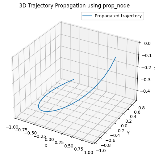

Compute Error

source

jacobi_test

 jacobi_test (X:numpy.ndarray, mu:float)

Compute the energy error. X can have either 6 columns (state vector) or 7 columns (time + state vector). The returned quantity is the cumulative error with respect to the initial value. If propagation is perfect, err = 0 (or very small).

	Type	Details
X	ndarray	State vector with shape (n, 6) or (n, 7), where n is the number of samples
mu	float	Gravitational parameter
Returns	float

source

dynamics_defect

 dynamics_defect (X:numpy.ndarray, mu:float)

Compute the dynamical defect for the generated time-state sequence. The returned quantity is the cumulative error on the position and velocity components. The overall metrics can be a combination of these two last errors.

	Type	Details
X	ndarray	Time-state vector with shape (n, 7), where the first column is the time vector
mu	float	Gravitational parameter
Returns	Tuple

# Select a random orbit from the dataset
num_orbits, num_components, num_time_points = orbit_data.shape  # Should be (400, 7, 100)
random_orbit_index = np.random.randint(0, num_orbits)
selected_orbit = orbit_data[random_orbit_index, :, :]

# The time vector is already included as the first component
# No need to add time column since data is already (400,7,100)
time_state_vector = selected_orbit.T  # Transpose to get (100,7) shape needed for dynamics_defect

# Test jacobi_test function
energy_error = jacobi_test(time_state_vector, mu)  # Pass all 7 columns since jacobi_test handles both cases
print("Cumulative energy error for the selected orbit:", energy_error)

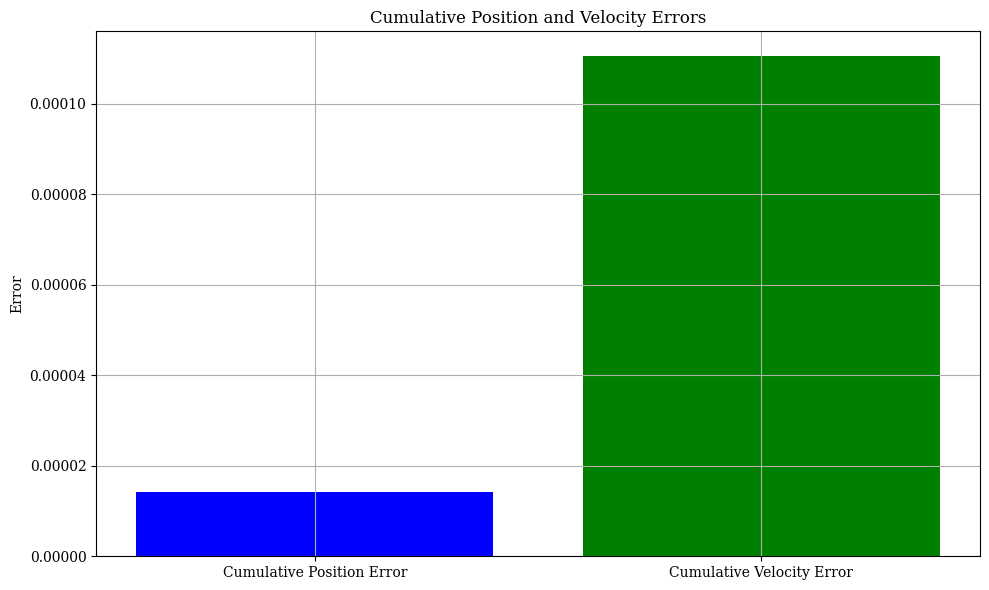
# Test dynamics_defect function
pos_error, vel_error = dynamics_defect(time_state_vector, mu)
print("Cumulative position error for the selected orbit:", pos_error)
print("Cumulative velocity error for the selected orbit:", vel_error)

# Visualize the numerically propagated orbit
visualize_static_orbits(orbit_data, time_instants=[0, 25, 50, 75], orbit_indices=[random_orbit_index])

# Visualize the cumulative errors calculated
fig, ax = plt.subplots(figsize=(10, 6))

labels = ['Cumulative Position Error', 'Cumulative Velocity Error']
errors = [pos_error, vel_error]

ax.bar(labels, errors, color=['blue', 'green'])
ax.set_ylabel('Error')
ax.set_title('Cumulative Position and Velocity Errors')
ax.grid(True)

plt.tight_layout()
plt.show()

Cumulative energy error for the selected orbit: 0.00018692017
Cumulative position error for the selected orbit: 1.4306169667270132e-05
Cumulative velocity error for the selected orbit: 0.00011048713047470115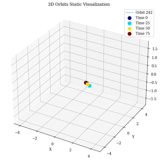

source

calculate_errors

 calculate_errors (orbit_data:numpy.ndarray, mu:float,
                   orbit_indices:List[int]=None,
                   error_types:List[str]=['position', 'velocity',
                   'energy'], time_step:Optional[float]=None,
                   display_results:bool=True, cumulative:bool=False)

Calculate and return the cumulative error and the average error per time step for the selected orbits together. Optionally, display the evolution of each error as a chart.

	Type	Default	Details
orbit_data	ndarray		3D array of orbit data
mu	float		Gravitational parameter
orbit_indices	List	None	List of integers referring to the orbits to analyze
error_types	List	[‘position’, ‘velocity’, ‘energy’]	Types of errors to calculate
time_step	Optional	None	Optional time step if time dimension is not included
display_results	bool	True	Boolean to control whether to display the results
cumulative	bool	False	Boolean to control cumulative or average error
Returns	Dict

errors = calculate_errors(orbit_data, EM_MU, orbit_indices = [0, 1, 2])

Cumulative position error for selected orbits: 0.0014242519694434052
Average position error per time step: 4.7954611765771215e-06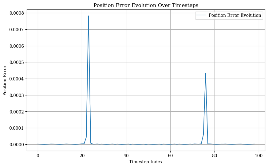

Cumulative velocity error for selected orbits: 0.0798643959065006
Average velocity error per time step: 0.00026890368992087745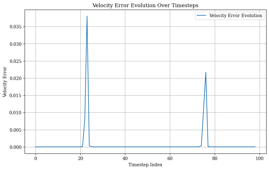

Cumulative energy error for selected orbits: 0.06817007064819336
Average energy error per time step: 0.00022952885774429888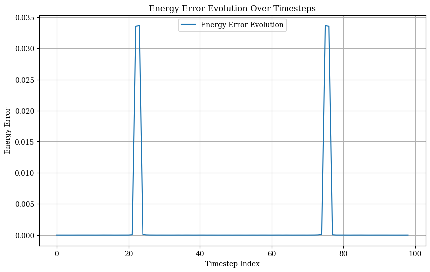

source

calculate_errors_per_orbit

 calculate_errors_per_orbit (orbit_data:numpy.ndarray, mu:float,
                             error_types:List[str]=['position',
                             'velocity', 'energy'],
                             time_step:Optional[float]=None,
                             display_results:bool=False)

Calculate and return the average error per orbit for the selected error types. Optionally, display the evolution of each error as a chart.

	Type	Default	Details
orbit_data	ndarray		3D array of orbit data
mu	float		Gravitational parameter
error_types	List	[‘position’, ‘velocity’, ‘energy’]	Types of errors to calculate
time_step	Optional	None	Optional time step if time dimension is not included
display_results	bool	False	Boolean to control whether to display the results
Returns	Dict

errors = calculate_errors_per_orbit(orbit_data[0:3], EM_MU, display_results=True)

Average Position Error per Orbit:
[5.14651324e-07 3.51359548e-07 1.35203727e-05]
Average Velocity Error per Orbit:
[1.81187043e-06 1.44955704e-06 8.03449642e-04]
Average Energy Error per Orbit:
[3.79543121e-06 2.81285747e-06 6.81978301e-04]