Latent Space

Scripts to visualize and explore the Latent Space

Plot 2 dimensions

plot_2d_latent_space

 plot_2d_latent_space (latent_representations:numpy.ndarray,
                       labels:numpy.ndarray,
                       latent_stdevs:Optional[numpy.ndarray]=None,
                       features:Optional[Any]=None,
                       feature_names:Optional[List[str]]=None,
                       figsize:tuple=(12, 12),
                       save_path:Optional[str]=None,
                       many_classes:bool=False, show_legend:bool=True,
                       legend_fontsize:int=8, plot_std:bool=True,
                       title:Optional[str]='2D Latent Space
                       Visualization', title_size:int=14,
                       axis_labels:Optional[Tuple[str,str]]=('Dimension
                       1', 'Dimension 2'), normalize_data:bool=True,
                       **kwargs:Any)

*Plots a 2D latent space visualization with class labels and feature distributions.

Parameters: - latent_representations: np.ndarray, shape (n_samples, 2) The 2D coordinates of the latent representations. - labels: np.ndarray, shape (n_samples,) The class labels for each sample. - features: Optional[Any], shape (n_samples, n_features) The feature data to plot distributions. Can be a list or a NumPy array. - feature_names: Optional[List[str]] The names of the features. - figsize: tuple, default (12, 12) The size of the entire figure. - save_path: Optional[str] Path to save the figure. If None, the plot is not saved. - many_classes: bool, default False If True, uses different markers for classes. - show_legend: bool, default True If True, displays legends. - legend_fontsize: int, default 8 Font size for the legends. - plot_std: bool, default True If True, plots the standard deviation shading for feature distributions. - title: Optional[str], default ‘2D Latent Space Visualization’ Title of the plot. - title_size: int, default 14 Font size for the title. - axis_labels: Optional[Tuple[str, str]], default (‘Dimension 1’, ‘Dimension 2’) Labels for the X and Y axes. - normalize_data: bool, default False If True, normalizes the latent representations. - kwargs: Any Additional keyword arguments passed to scatter plots.*

	Type	Default	Details
latent_representations	ndarray
labels	ndarray
latent_stdevs	Optional	None
features	Optional	None
feature_names	Optional	None
figsize	tuple	(12, 12)
save_path	Optional	None
many_classes	bool	False
show_legend	bool	True
legend_fontsize	int	8
plot_std	bool	True
title	Optional	2D Latent Space Visualization	New title parameter
title_size	int	14	New title_size parameter
axis_labels	Optional	(‘Dimension 1’, ‘Dimension 2’)	New axis_labels parameter
normalize_data	bool	True	New parameter to control normalization
kwargs	Any
Returns	None

source

plot_combined_2d_latent_space

 plot_combined_2d_latent_space (real_latent:numpy.ndarray,
                                synthetic_latent:numpy.ndarray, synthetic_
                                labels:Union[int,List[int],numpy.ndarray,N
                                oneType]=None, figsize:tuple=(12, 9),
                                save_path:Optional[str]=None,
                                show_legend:bool=True,
                                axis_labels:tuple=('X-axis', 'Y-axis'),
                                title:Optional[str]=None,
                                colormap:str='viridis',
                                feature_title:Optional[str]='Feature
                                Value', label_names:Optional[dict]=None)

*Plots the combined latent space of real and synthetic data. Assumes the latent space is 2D. If synthetic_latent is a 3D array, it plots arrows. Numeric annotations for arrows are only displayed if synthetic_labels are provided.

Args: real_latent (np.ndarray): Latent representations of real data. synthetic_latent (np.ndarray): Latent representations of synthetic data or arrows. synthetic_labels (Optional[Union[int, List[int], np.ndarray]]): Labels for synthetic data. Can be None, a single label, or a list of labels. figsize (tuple): Size of the figure. save_path (Optional[str]): Optional path to save the plot image. show_legend (bool): Flag to show or hide the legend. axis_labels (tuple): Labels for the X and Y axes. title (Optional[str]): Title of the plot. colormap (str): Colormap to use when coloring by features. feature_title (Optional[str]): Title for the feature color bar. label_names (Optional[dict]): Dictionary mapping label values to names for discrete labels.

Returns: None*

	Type	Default	Details
real_latent	ndarray		Latent representations of real data.
synthetic_latent	ndarray		Latent representations of synthetic data or arrows.
synthetic_labels	Union	None	Labels for synthetic data. Can be None, a single label, or a list of labels.
figsize	tuple	(12, 9)	Size of the figure.
save_path	Optional	None	Optional path to save the plot image.
show_legend	bool	True	Flag to show or hide the legend.
axis_labels	tuple	(‘X-axis’, ‘Y-axis’)	Labels for the X and Y axes.
title	Optional	None	Title of the plot.
colormap	str	viridis	Colormap to use when coloring by features.
feature_title	Optional	Feature Value	Title for the feature color bar.
label_names	Optional	None	New parameter: dictionary mapping label values to names
Returns	None

Reduce dimensions

source

reduce_dimensions_latent_space

 reduce_dimensions_latent_space (latent_representations:numpy.ndarray,
                                 labels:numpy.ndarray,
                                 techniques:List[str]=['PCA'],
                                 n_components:int=2, figsize:tuple=(12,
                                 9), save_path:Optional[str]=None,
                                 many_classes:bool=False,
                                 grid_view:bool=True,
                                 class_names:Optional[List[str]]=None,
                                 show_legend:bool=True, plot:bool=True,
                                 **kwargs:Any)

*Reduces dimensions of latent representations using specified techniques and optionally plots the results.

Returns: A dictionary containing the reduced latent space for each technique.*

	Type	Default	Details
latent_representations	ndarray		Precomputed latent representations (numpy array).
labels	ndarray		Labels for the data points, used for coloring in the plot.
techniques	List	[‘PCA’]	Techniques to use for reduction (‘PCA’, ‘t-SNE’, ‘UMAP’, ‘LDA’).
n_components	int	2	Number of dimensions to reduce to (1, 2, or 3).
figsize	tuple	(12, 9)	Size of the figure for each subplot.
save_path	Optional	None	Optional path to save the plot image.
many_classes	bool	False	Flag to use enhanced plotting for many classes.
grid_view	bool	True	Flag to plot all techniques in a single grid view.
class_names	Optional	None	Optional class names for the legend
show_legend	bool	True	Flag to show or hide the legend
plot	bool	True	Flag to plot the latent space
kwargs	Any
Returns	Dict		Additional keyword arguments for dimensionality reduction methods.

source

reduce_dimensions_combined_latent_space

 reduce_dimensions_combined_latent_space (train_latent:numpy.ndarray,
                                          val_latent:numpy.ndarray, train_
                                          labels:Optional[numpy.ndarray]=N
                                          one,
                                          techniques:List[str]=['PCA'],
                                          n_components:int=2,
                                          **kwargs:Any)

*Reduces dimensions of latent representations using specified techniques.

Returns: A dictionary containing the reduced latent space for each technique and dataset (train and val).*

	Type	Default	Details
train_latent	ndarray		Latent representations of training data.
val_latent	ndarray		Latent representations of validation data.
train_labels	Optional	None	Labels for the training data points (optional for LDA).
techniques	List	[‘PCA’]	Techniques to use for reduction (‘PCA’, ‘t-SNE’, ‘UMAP’, ‘LDA’).
n_components	int	2	Number of dimensions to reduce to (1, 2, or 3).
kwargs	Any
Returns	Dict		Additional keyword arguments for dimensionality reduction methods.

from orbit_generation.data import get_example_orbit_data

orbit_data = get_example_orbit_data()
orbit_data.shape

# Reshape data to 2D (num_orbits, 6 * num_time_points)
orbit_data_reshaped = orbit_data.reshape(200, -1)

# Use PCA to reduce to a lower-dimensional space (e.g., 10 dimensions)
pca = PCA(n_components=10)
latent_representations = pca.fit_transform(orbit_data_reshaped)

labels = np.random.randint(0, 5, size=200)  # 5 different classes

reduced_latent_spaces = reduce_dimensions_latent_space(latent_representations, labels, techniques=['UMAP','LDA'])
reduced_latent_spaces['UMAP'].shape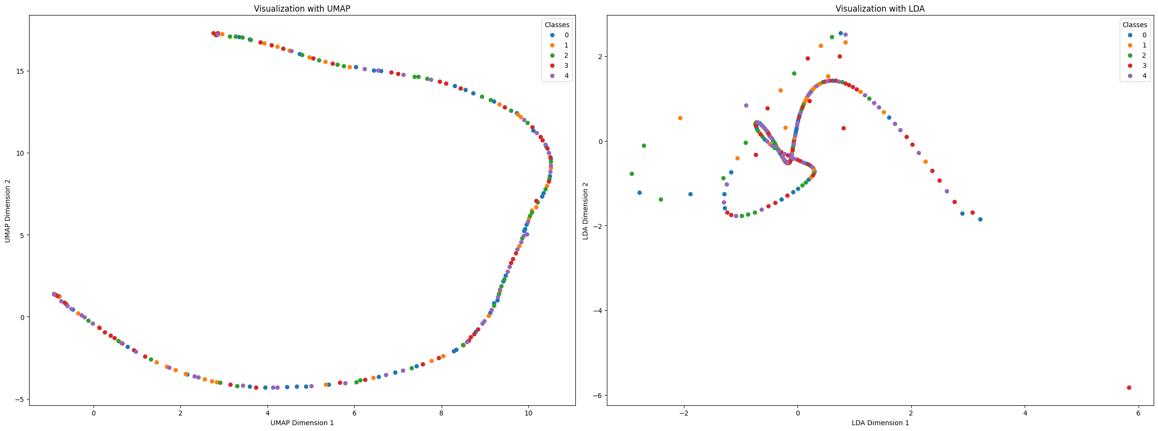

reduced_latent_spaces=reduce_dimensions_latent_space(latent_representations, labels, techniques=['PCA'], n_components=1, many_classes=True)
reduced_latent_spaces['PCA'].shape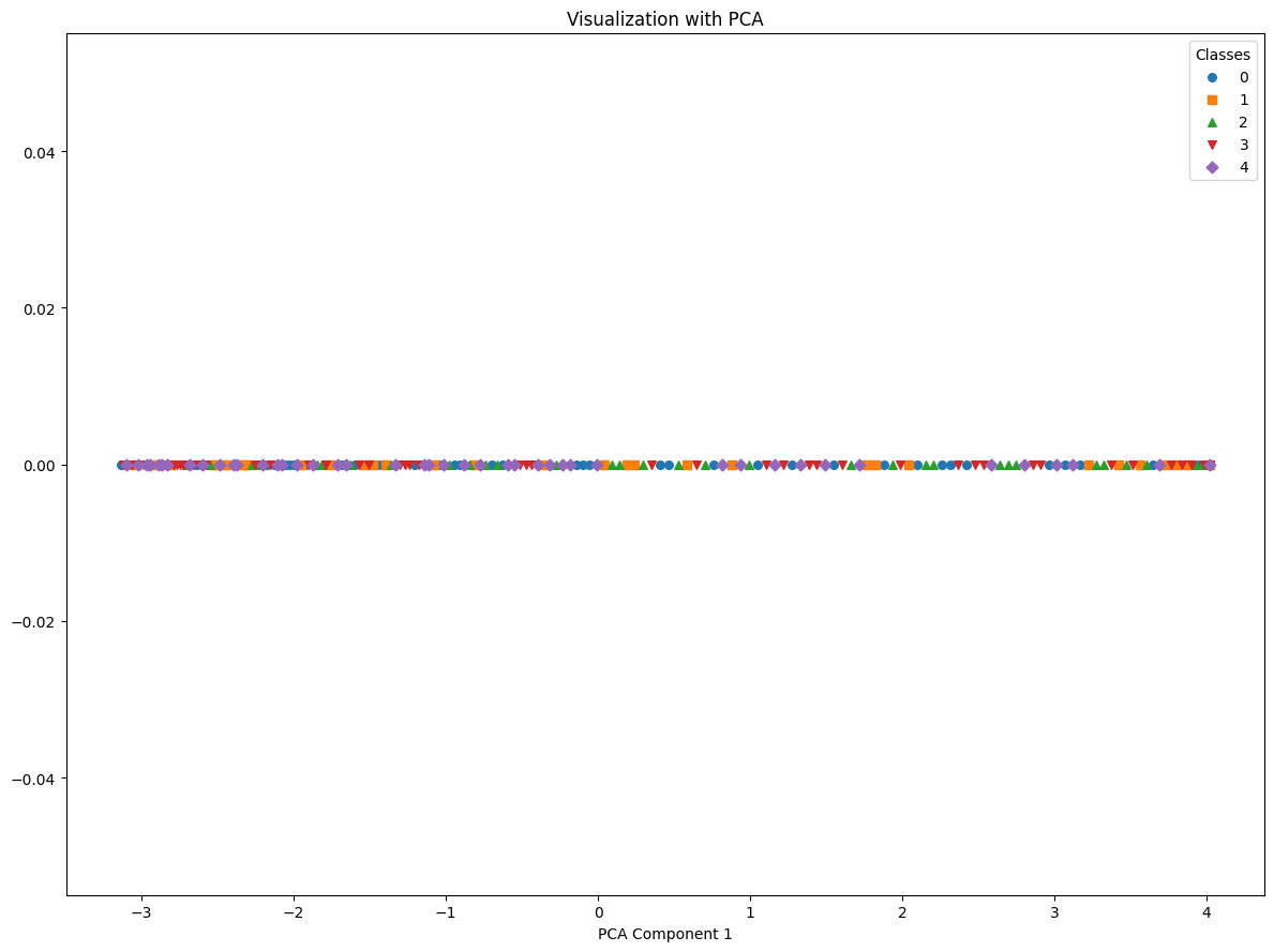

reduced_latent_spaces=reduce_dimensions_latent_space(latent_representations, labels, techniques=['t-SNE'], n_components=3)
reduced_latent_spaces['t-SNE'].shape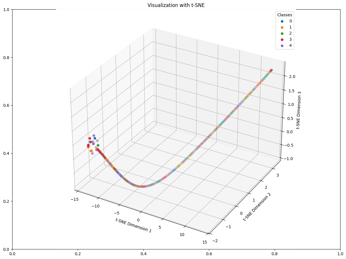

Sampling

source

sample_random_distributions

 sample_random_distributions (means, log_vars, n_samples:int,
                              log_var_multiplier:float=1.0)

source

interpolate_sample

 interpolate_sample (centroids, granularity=10, variance=0.0)

*Perform interpolating sampling between all pairs of centroids.

Parameters: - centroids (np.ndarray): Array of shape (n_centroids, latent_dim). - granularity (int): Number of interpolation steps between each pair. - variance (float): Standard deviation for Gaussian sampling.

Returns: - samples (np.ndarray): Array of sampled points.*

source

slerp

 slerp (z1, z2, steps)

Perform spherical linear interpolation between two points.

source

linear_interpolation

 linear_interpolation (z1, z2, steps)

Perform linear interpolation between two points.

# Define example centroids for a 2-dimensional latent space
centroids = np.array([
    [1.0, 2.0],
    [3.0, 4.0],
    [5.0, 6.0]
])

granularity = 3
variance = 0.0  # Set to 0 for deterministic interpolation

sampled_points = interpolate_sample(centroids, granularity, variance)

# Define the expected sampled points manually for granularity=3
expected_data = np.array([
    [1.0, 2.0],
    [2.0, 3.0],
    [3.0, 4.0],
    [1.0, 2.0],
    [3.0, 4.0],
    [5.0, 6.0],
    [3.0, 4.0],
    [4.0, 5.0],
    [5.0, 6.0]
])

# Check the sampled points against the expected data
test_eq(sampled_points, expected_data)

source

grid_sample

 grid_sample (encodings:numpy.ndarray,
              grid_size:Union[int,Tuple[int,...]]=100)

def visual_test():
    # Generate random encodings
    np.random.seed(42)
    encodings = np.random.rand(100, 2) * 100  # 100 points in a 100x100 space

    # Perform grid sampling
    grid_size = (10, 10)
    sampled_grid = grid_sample(encodings, grid_size)

    # Calculate bounds for visualization
    x_min, y_min = np.min(encodings, axis=0)
    x_max, y_max = np.max(encodings, axis=0)

    # Plot the encodings
    plt.figure(figsize=(8, 8))
    plt.scatter(encodings[:, 0], encodings[:, 1], c='blue', label='Encodings')

    # Plot the sampled grid points
    plt.scatter(sampled_grid[:, 0], sampled_grid[:, 1], c='red', marker='o', label='Sampled Grid Points')

    # Draw grid lines for reference
    x_edges = np.linspace(x_min, x_max, grid_size[0] + 1)
    y_edges = np.linspace(y_min, y_max, grid_size[1] + 1)

    plt.title('Grid Sampling Visualization with Sampled Grid Points')
    plt.xlabel('X-axis')
    plt.ylabel('Y-axis')
    plt.legend()
    plt.grid(False)
    plt.show()

# Run the visual test
visual_test()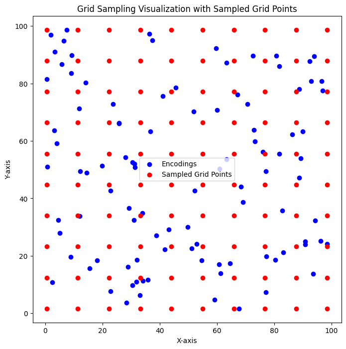

Explore

source

trimmed_mean_centroid

 trimmed_mean_centroid (points, trim_ratio=0.1)

source

compute_medoid

 compute_medoid (points)

source

geometric_median

 geometric_median (points, tol=1e-05)

source

compute_centroids

 compute_centroids (latents, labels, method='mean', return_labels=False,
                    **kwargs)

*Compute the centroid of each class in the latent space using various methods.

Parameters: - latents (np.ndarray): Array of shape (n_samples, latent_dim). - labels (np.ndarray): Array of shape (n_samples,) with class labels. - method (str): Method to compute centroids. Options: ‘mean’, ‘median’, ‘geom_median’, ‘medoid’, ‘trimmed_mean’, ‘gmm’. - return_labels (bool): If True, also return the unique labels corresponding to the centroids. - kwargs: Additional arguments for specific methods.

Returns: - centroids (np.ndarray): Array of shape (n_classes, latent_dim) containing centroids. - unique_labels (np.ndarray, optional): Array of shape (n_classes,) with unique class labels.*

Measure

source

plot_linear_regression

 plot_linear_regression (latent_means, features, feature_names,
                         normalize=False)

*Perform linear regression for each feature, visualize the results, and return regression metrics.

Parameters: - latent_means: np.ndarray of shape (n_samples, latent_dim), the latent space coordinates. - features: np.ndarray of shape (n_samples, n_features), the feature values. - feature_names: List of strings representing the names of the features. - normalize: Boolean, whether to normalize the features and latent space (default: False).

Returns: - results: Dictionary containing coefficients, intercepts, and R² values for each feature. - simple_results: Dictionary containing R² values for each feature with modified keys.*